
Generative Augmentation in Sparse Data Regimes: A Controlled Factorial Study in Chinese Character Classification
Teaching a machine to read Chinese
The Chinese writing system has tens of thousands of characters. Each one is a small, precise arrangement of strokes. To teach a computer to recognize even a single character, you need many labeled examples of it: handwritten, varied, each tagged with the right answer.
That is the catch. Collecting and labeling those examples is slow and expensive. And when a model has too few of them, it does not learn the character. It memorizes. It learns the exact pixels in the handful of images it was shown, then falls apart the moment it sees a new one. This is called overfitting. The model is brilliant on the practice test and helpless on the real thing.
An idea: let the model invent its own examples
There is a standard fix for too little data. You make more of it.
The simple version rotates, flips, and crops the images you already have. It helps. But it is bounded. Every new image is just a warped copy of an old one.
The ambitious version is stranger. You train a second model to learn what the characters look like, the shapes and proportions and the logic of the strokes. Then you ask it to draw new ones. Not copies. New characters it has never seen, but that look like they belong.
The model that does the drawing is a GAN, a generative adversarial network. Picture two networks locked in a game. One is a forger, painting fake characters. The other is a detective, trying to tell the fakes from the real ones. They train against each other. The forger keeps losing, but slowly improving until, finally, its fakes are good enough to fool the detective. By then the forger has learned to produce convincing characters on demand. The exact version I used is a Wasserstein GAN with a gradient penalty. That is just a flavor that trains far more steadily than the original. I will call it the generator, and I will call the detective the critic. Remember the critic. It comes back later.
A first look, and a trap
To test the idea I used Chinese-MNIST, a Chinese-character version of the classic MNIST (Modified National Institute of Standards and Technology) handwritten-digit benchmark. It has fifteen characters: the digits zero through nine plus five magnitude characters like ten and thousand, with a thousand small grayscale images each. To simulate scarcity, I held most of them back and trained on a thin slice per class. The classifier I trained on that slice was a plain convolutional network. Nothing fancy.
I started with two experiments.
In the first, I gave the classifier fifty real images per class to train with. It reached 88.5% accuracy. Then I mixed in synthetic characters from the generator, raw and uncurated. Accuracy slipped a point or two. The fakes had made it worse.
In the second, I starved the classifier: I gave it only twenty-five real images per class to train on, half as many examples as before. This time, before adding the synthetic images, I filtered them. I used the critic as a judge, kept only its top-rated fakes, and threw the rest away. Now accuracy jumped, from 71.8% up to around 80%. The filtered fakes had helped, and helped a lot.
Put the two together and the moral seems obvious. Raw synthetic data hurts. Filtered synthetic data helps. The filter is the magic. Curate your fakes and augmentation pays off.
It is a tidy story. It is also wrong. And the way it is wrong is the interesting part.
What changed twice
Look again at what I did. Between the first experiment and the second, I changed two things at the same time.
The first had plenty of data and no filter. The second had scarce data and a filter. So when the result flipped, from “synthetic data hurts” to “synthetic data helps,” what caused the flip? The filter I added? Or the scarcity I imposed? The two moved together, in lockstep. There is no way to separate them after the fact.
This is a confound, and it is the oldest trap in experimental design. When two things change at once, you cannot hand the credit to either one.
Maybe the filter was doing all the work. Or maybe, and this is the possibility I had not taken seriously, the filter was doing nothing. Maybe augmentation helped in the second experiment for a much duller reason: a starved classifier has room to grow, and a well-fed one does not. From those two experiments alone, both explanations fit the numbers perfectly. The data could not tell them apart.
There is only one cure. Change one thing at a time.
Changing one thing at a time
So I built the full grid and ran every combination.
There are three knobs. How much real data: twenty-five or fifty images per class. Whether I filter the synthetic data or not. And how much synthetic data I mix in: one fake per real image, or four. Every combination, plus a plain baseline at each data level with no synthetic data at all.
One rule makes the whole thing honest. The filtered and unfiltered fakes were drawn from the same pool of generated images. The only difference was whether I kept the critic’s top picks or a random handful. Same generator, same pool, one knob moving at a time.
This is a factorial design, and breaking confounds apart is exactly what it is for. Now I could ask two clean questions instead of one muddled one. Hold the filter fixed and vary the data: what does scarcity do? Hold the data fixed and vary the filter: what does the filter do?
Here is the full ledger.
| Real images / class | Condition | Accuracy (%) | Change vs. baseline (%) | p-value |
|---|---|---|---|---|
| 25 | Baseline (no synthetic) | 71.77 | — | — |
| Unfiltered, 1:1 | 77.52 | +5.75 | 0.005 | |
| Unfiltered, 4:1 | 78.79 | +7.01 | 0.003 | |
| Filtered, 1:1 | 77.88 | +6.11 | 0.007 | |
| Filtered, 4:1 | 79.01 | +7.24 | 0.004 | |
| 50 | Baseline (no synthetic) | 88.49 | — | — |
| Unfiltered, 1:1 | 87.05 | −1.44 | 0.049 | |
| Unfiltered, 4:1 | 86.35 | −2.15 | 0.009 | |
| Filtered, 1:1 | 87.60 | −0.89 | 0.222 | |
| Filtered, 4:1 | 86.48 | −2.01 | 0.001 |
The controlled re-run reproduced both baselines exactly, 88.5% and 71.8%, which is a small but reassuring sign that the whole thing is repeatable.
Read the ledger in two blocks. The bottom block is the well-fed classifier, fifty images per class. Its baseline is already high. Look what synthetic data does to it: every single row is negative. Filtered or not, one-to-one or four-to-one, the fakes drag it down. A classifier with enough real data does not want your inventions.
The top block is the starved classifier, twenty-five per class. Its baseline accuracy is a shaky 71.8%. Here every row is positive. Synthetic data lifts it by six or seven points, and the more you add, the higher it climbs. The best case buys back 7.2 of the 16.7 points I had lost by halving the data. That is about 43% of the damage undone, without having to add any new real data!
So the first question answers itself, and loudly. Whether augmentation helps or hurts is decided almost entirely by one thing: are you data-starved or not? Starved, it helps. Comfortable, it hurts.
The filter I was sure about
Now the second question. The one I had built the whole project around. Did the filter help?
To ask it cleanly, you compare filtered against unfiltered at the same data level and the same ratio. That holds everything else still and lets the filter be the only thing moving. There are four such comparisons. Here is what the filter bought in each:
- Fifty per class, one-to-one: filtered won by 0.55 points.
- Fifty per class, four-to-one: by 0.13 points.
- Twenty-five per class, one-to-one: by 0.36 points.
- Twenty-five per class, four-to-one: by 0.23 points.
The largest gap is barely half a point. Set that against the six- and seven-point swings from scarcity, and it is a rounding error.
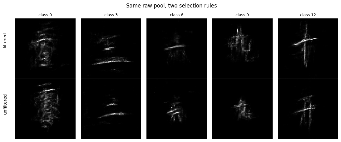
So I went back to the images, expecting to find the explanation there. I expected the filtered set to look clearly better than the random one. It does not. The critic’s top-scored characters are only a little cleaner than a random handful from the same pool. And neither set looks good. Both are ratty: broken strokes, smears, characters that wobble between two shapes. The generator simply is not strong enough, and skimming off its best few percent does not rescue much. The “good” pile and the “whatever” pile look almost the same, and both look rough.
Once you see that, the weak result stops being mysterious. A filter that barely changes the images can only barely change the outcome. I was not watching high-quality data fail to help. I was watching mediocre data get swapped for slightly-less-mediocre data, and getting, predictably, a barely different result.
One number in that list still deserves a second look, because it hides a trap of its own. The first comparison, fifty per class at one-to-one, came in at p = 0.034. By the usual convention, anything under 0.05 counts as a real effect. On its face, this says the filter did help there. Should I believe it?
No, and the reason is worth understanding. I did not run one comparison. I ran four, and then picked out the smallest p-value. Giving yourself four tries and reporting the best one is like buying four lottery tickets and being amazed that one of them won. With enough tickets, something always hits, even when every ticket is a long shot. So when you make several comparisons, you have to raise the bar for what counts as real.
The Holm–Bonferroni correction is one standard way to raise it. The idea is plain. Divide your threshold by the number of comparisons. Four comparisons turn the old 0.05 bar into about 0.0125. My p = 0.034 clears the old bar easily and slams into the new one. It does not survive. Once you account for the fact that I went fishing through four results, that lone “significant” effect dissolves.
So here is the honest verdict, and it is sharper than “the filter does nothing.”
Per condition, the filter is invisible. None of the four filtered-versus-unfiltered comparisons is significant on its own, and the one that looked significant does not survive the correction above.
But the per-condition view throws one thing away: direction. All four comparisons favor filtering. So does every one of the five seeds, once you average its filter effect across the four conditions. That much agreement is itself evidence. Pool the four comparisons properly and the consistency becomes a number: a small but real positive effect of about a third of a percentage point, every seed pointing the same way, sitting right on the edge of statistical significance.
So the filter is not doing nothing. It is doing almost nothing: a genuine, repeatable nudge, far too small to matter beside the six- or seven-point swing from scarcity. And the reason it is so small is the one the pictures already gave away. Stage one barely improved the images, so it could only barely improve the result. And there is something satisfying in that. The effect came out exactly as small as its cause.
The pooled analysis, including what “properly” means and the borderline p-value it lands on, is in the appendix below.
Where the hope is
This is exactly why I keep saying stage one.
The filter I designed has two stages, and I only built the first. Stage one is the critic: rank the fakes by how real they look, keep the top ones. We just saw what it does, which is to say, not much, because its top picks are not much better than the rest.
Stage two is a different kind of check, and a stricter one. Instead of trusting the critic’s single realism score, it compares each synthetic character directly against real characters of the same class. It uses two perceptual measures. The first, the Structural Similarity Index Measure (SSIM), asks how closely the structure of two images matches. The second, Learned Perceptual Image Patch Similarity (LPIPS), asks how close they sit in the feature space of a network trained to see the way people do. It is built to throw out the images that pass the critic but are subtly the wrong shape. Plausible at a glance, wrong on inspection.
And that is the hopeful part. Stage one helped only negligibly, because it barely sorted good from bad. A filter that actually separates them, strict enough to leave you with characters that look genuinely right rather than just least-wrong, is a different experiment, and an untested one. The door on quality filtering is not closed. I just have not yet built the filter that would knock on it properly.
What it means
Two things come out of this.
The practical one is for anyone working with scarce data, including the real prize behind all of this: fields like medical imaging, where every label is hard-won. Augmentation is not a free upgrade you sprinkle on everything. It depends entirely on your regime. If you are truly starved, augment. And for now, do not bother filtering, because the simple filter does not earn its keep. If you already have enough data, synthetic data will quietly cost you. The first question is not how should I curate my fakes. It is am I actually starved, and only if you are, augment.
The deeper lesson is the one I almost missed. My first two experiments told a clean, satisfying, completely wrong story. They did it precisely because they changed two things at once. That is worth sitting with. A confounded experiment does not just fail to find the answer. It can hand you a convincing wrong one: a mechanism that looks real and is not. The fix was not clever. It was the dullest discipline there is. Change one thing at a time. Old advice, easy to skip, and easiest of all to skip when the wrong answer is the one you were hoping to find.
Under the hood
For the reader who wants the specifics:
- Generator. A conditional Wasserstein GAN with gradient penalty, trained for 500 epochs. The Wasserstein-with-gradient-penalty recipe is what kept training stable.
- The filter, stage one, the part actually tested. For each character, one pool of 800 generated images, each scored once by the trained critic. Filtered keeps the top-scored images, between roughly the top 3% and the top 25% of the pool depending on how many were needed. Unfiltered takes a random draw from that same pool. Stage two, the perceptual screen, was never built.
- Classifier. A plain three-block convolutional network, held identical across every condition, so that any difference traces to the data and not the model.
- The runs. Five random seeds per condition, so every number above is a mean with a real spread behind it. Because all conditions share the same five seeds, each seed forms a matched pair, which lets a paired t-test cancel the run-to-run noise and compare treatments directly.
- Significance. Paired t-test, threshold 0.05.
Appendix: did filtering help, really?
The four filtered-versus-unfiltered comparisons in the body were all positive but, one at a time, unconvincing. Does their shared direction add up to something real once pooled? Here is the check.
The inputs are the per-seed accuracies behind every cell of the ledger: ten conditions, five seeds each, fifty classifier trainings in all. The four isolation comparisons (filtered − unfiltered, paired by seed, at fixed real-count and ratio) are:
| Comparison | Filter effect (pp) | Paired-t p |
|---|---|---|
| 50/class, 1:1 | +0.55 | 0.034 |
| 50/class, 4:1 | +0.13 | 0.78 |
| 25/class, 1:1 | +0.36 | 0.55 |
| 25/class, 4:1 | +0.23 | 0.64 |
All positive; none significant after correcting for the four looks. To pool them, I averaged each seed’s filter effect across the four conditions. Because the same five seeds run through every condition, that yields five independent per-seed estimates of the average effect: +0.27, +0.18, +0.37, +0.67, +0.10 pp — every one positive.
A one-sample t-test on those five (the appropriate test, since the seed is the independent unit) gives a mean of +0.32 pp, 95% CI [+0.04, +0.59], t = 3.21 (df = 4), p = 0.033. Two distribution-free checks — a Wilcoxon signed-rank test and an exact sign-flip permutation — both give p = 0.063. The effect sits right on the 0.05 line: significant parametrically, just shy of it without.
One shortcut is wrong: treating all twenty paired differences as independent gives p = 0.13 and finds nothing. The twenty are not independent (five share each seed), and that false inflation buries the signal; averaging within each seed first respects the structure and recovers it.
Two caveats keep it modest. The effect, about a third of a percentage point, is negligible beside the six- to seven-point scarcity swing. And the seeds randomize only classifier training, not the generator or the synthetic pool, both fixed here — so this is a tiny consistent edge for this generator and this pool, not a claim that it generalizes. The verdict: a small, consistent, borderline-significant positive effect, real and repeatable, and still too small to act on.
The work
- Research Paper (PDF)
- Jupyter Notebook
- Pooled-analysis notebook
- Course: EN.705.603 Introduction to Generative AI, Johns Hopkins University, Spring 2026